Eulerian/Lagrangian Coupling (ELC) Documentation
Introduction
This package handles the communication between the Lagrangian solid solver and the Eulerian fluid solver in the vtf_page.
This is a templated class library. Thus there is no library to compile or link with. Just include the appropriate header files in your application code when you compile.
When the Lagrangian solvers have a solid mesh, the boundary of the mesh is communicated to the Eulerian solvers and the fluid pressures at the boundary nodes are communicated back to the Lagrangian solvers. The elc::LagrangianCommBoundary and elc::EulerianCommBoundary classes implement point-to-point communication between the solid and fluid.
When the Lagrangian solvers have a shell, the shell is sent to the Eulerian solvers and the pressure differences across the shell faces are sent back. The elc::LagrangianCommShell and elc::EulerianCommShell classes implement the point-to-point communication in this case.
The Coupled Simulation
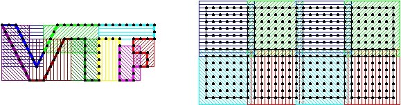
In the coupled Eulerian/Lagrangian VTF simulation, the solid mesh and the fluid grid are each distributed over a number of processors. The typical VTF simulation is in 3-D and uses an AMR (Adaptive Mesh Refinement) fluid grid. For the sake of simplicity, we will illustrate everything in 2-D with a unigrid fluid mesh. We consider the case of a 2-D solid (instead of a shell). Below we show a 2-D diagram of a solid mesh and a fluid grid. We indicate how the fluid grid is distributed over 8 processors.
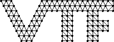
Solid mesh.
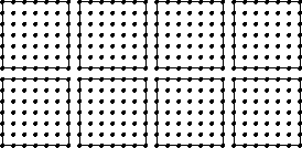
Fluid grid.
At each time step, the fluid needs the position and velocity of the solid boundary. This is used in the Ghost Fluid Method (GFM) to enforce boundary conditions at the solid/fluid interface. In return, the solid solvers need the fluid pressure at the boundary nodes.
The solid mesh is distributed. Below we show a distribution of the boundary over 9 processors.
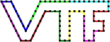
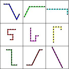
The distributed solid boundary.
The Gather-Send-Broadcast Algorithm
Before presenting the point-to-point coupling algorithm used in ELC, we introduce a simple coupling algorithm. One way of communicating the solid boundary to the fluid processors is the gather-send-broadcast algorithm. The process is illustrated below. 9 solid processors communicate the solid boundary to 8 fluid processors.
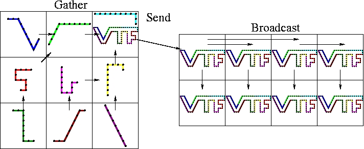
The gather-send-broadcast algorithm.
The gather-send-broadcast algorithm communicates the solid boundary to the fluid in three steps:
- Gather. The solid processors perform a gather operation to collect the portions of the boundary to the root solid processor. There the pieces are sewn together to make one cohesive mesh.
- Send. The assembled boundary mesh is then sent to the root fluid processor.
- Broadcast. The fluid processors then perform a broadcast operation to send the assembled boundary to each fluid processor.
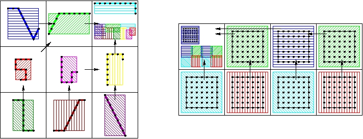
Each fluid processor can then select the portion of the assembled solid boundary that is relevant to its domain and use the closest point transform (CPT) to build the level set description of the boundary.
Communicating the fluid pressures to the solid is done with analogous operations:
- Gather. The fluid processors each set the pressure for the boundary nodes within their domain. Then a gather operation collects the pressures to the root.
- Send. The fluid root then sends the pressures on the assembled boundary to the solid root.
- Broadcast. The solid processors broadcast the pressures for the assembled boundary and then select the values for their portion of the boundary.
The gather-send-broadcast algorithm has a number of advantages:
- It is easy to implement.
- The number of communications is small.
- It does not depend on the distribution of the solid or fluid meshes.
The gather-send-brodcast is simple and flexible. However, for large problems it may have poor performance due to the need to assemble, store and communicate the global solid boundary. For the solid processors, assembling the global solid boundary may be costly (execution time) or infeasible (memory requirements) for large meshes. Note that each fluid processor receives the global boundary, though it only needs the portion that intersects its domain. Storing the global boundary may be infeasible; extracting the relevant portion of the boundary may be costly.
A Point-To-Point Communication Pattern
Now we present a point-to-point pattern for communicating the solid boundary and the fluid pressures at the boundary nodes. The communication pattern is determined by using bounding box information from the distributed solid boundary and fluid grids. (The point-to-point communication pattern is implemented in the Point-to-Point Bounding Box package.)
Each solid processor makes a bounding box around its portion of the boundary. Each fluid processor makes a bounding box that contains its region of interest. Any portion of the solid boundary in the region of interest could influence the fluid grid. These are illustrated below.
The solid and fluid bounding boxes.
The solid processors perform a gather operation to collect the bounding box information to the root. The fluid processors do the same.
Gather the solid and fluid bounding boxes.
Next the two root processors exchang the collected bounding boxes.
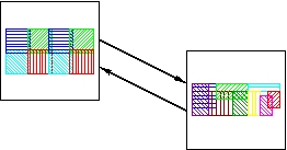
Exchange the collected solid and fluid bounding boxes.
Then the solid processors broadcast the fluid regions of interest and the fluid processors broadcast the solid boundary bounding boxes.
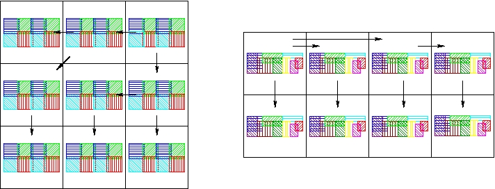
Broadcast the collected solid and fluid bounding boxes.
Now each solid processor has all the fluid regions of interest and each fluid processor has all the solid bounding boxes. Each solid processor finds the fluid regions of interest which overlap its bounding box. This determines the fluid processors to which it will send its portion of the boundary. Analogously, each fluid processor finds the solid bounding boxes which overlap its region of interest. This determines the solid processors from which it will receive portions of the boundary. The point-to-point communication from the solid to the fluid is illustrated below.
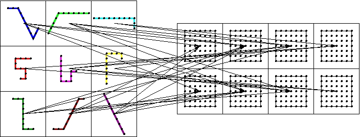
The point-to-point communication pattern.
Communicating with the Point-To-Point Scheme
Once the point-to-point communication pattern is determined (with the point-to-point bounding box package), each solid processor sends its portion of the boundary to the relevant fluid processors. Each fluid processor receives the relevant portions of the boundary and assembles these portions into a single cohesive mesh. It uses this mesh to compute the CPT. Then the pressure is determined at the nodes of the boundary mesh (with the Grid Interpolation/Extrapolation sub-package of the Numerical Algorithms package.) The pressures are then transfered to each portion of the boundary. Finally the pressures are sent back to the solid processor from whence the portion of the boundary came.
Like the gather-send-broadcast approach, the point-to-point communication scheme does not depend on any special distribution of the data. For reasonable data distributions, it has a number of advantages:
- It reduces the cost of assembling the boundary. Instead of assembling the entire boundary on the solid root, each fluid processor assembles only the relevant portion of the boundary.
- It reduces the storage overhead for the boundary. The global solid boundary is never assembled.
Usage on the Lagrangian Processors
In each Lagrangian processor, instatiate one of the ELC Lagrangian communicators.
elc::LagrangianComm<3,Number>
  lagrangianComm(MPI_COMM_WORLD, comm, numEulerian, eulerianRoot, elc::LocalIndices);
Here, Number is probably double, comm is the Lagrangian communicator, numEulerian is the number of Eulerian processors, and eulerianRoot is the rank of the root Eulerian processor in the world communicator. For the last argument one can either pass elc::LocalIndices or elc::GlobalIdentifiers. This indicates how one will specify the mesh in sendMesh(). The connectivities array may either contain indices of the local mesh, or global node identifiers.
To send the mesh to the Eulerian processors, do the following.
lagrangianComm.sendMesh(numNodes, identifiers, positions, velocities,
                        numFaces, connectivities);
lagrangianComm.waitForMesh();
Here, identifiers, positions, velocities, and connectivities are arrays of data that define the mesh. One can perform computations between sendMesh() and waitForMesh(). Upon completion of waitForMesh(), mesh array data has been copied into communication buffers, and thus the data may be modified.
To receive the pressure data from the Eulerian processors, use receivePressure() and waitForPressure(). Below we receive the pressure defined at the nodes.
lagrangianComm.receivePressure(numNodes, pressures);
lagrangianComm.waitForPressure();
If the Lagrangian mesh is a shell, then the pressure is defined at the centroids of the faces.
lagrangianComm.receivePressure(numFaces, pressures);
lagrangianComm.waitForPressure();
One can perform computations between receivePressure() and waitForPressure(). The former initiates non-blocking receives, so it is best to call this function before the Eulerian processors start sending the pressure.
Usage on the Eulerian Processors
In each Eulerian processor, instatiate one of the ELC Eulerian communicators. For coupling with the boundary of a solid mesh, use:
elc::EulerianCommBoundary<3,Number>
  eulerianComm(MPI_COMM_WORLD, comm, numLagrangian, lagrangianRoot, elc::LocalIndices);
For coupling with a shell mesh, use:
elc::EulerianCommShell<3,Number>
  eulerianComm(MPI_COMM_WORLD, comm, numLagrangian, lagrangianRoot, elc::LocalIndices);
Here, comm is the Eulerian communicator, numLagrangian is the number of Lagrangian processors, and lagrangianRoot is the rank of the root Lagrangian processor in the world communicator. For the last argument one can either pass elc::LocalIndices or elc::GlobalIdentifiers. This indicates how the mesh patches are specified in the Lagrangian processors' call to sendMesh(). There, the connectivities array may either contain indices of the local mesh, or global node identifiers.
To receive the mesh from the Lagrangian processors, do the following.
eulerianComm.receiveMesh(region);
eulerianComm.waitForMesh();
Here, region is an array of 6 floating point numbers that define the bounding box containing all of the processors' grids. One can perform computations between receiveMesh() and waitForMesh().
After setting the pressure with the getPressures() or the getPressuresData() member functions, send the pressure to the relevant Lagrangian processors.
eulerianComm.sendPressure();
eulerianComm.waitForPressure();
Generated on Thu Jun 30 02:14:53 2016 for Eulerian-Lagrangian Coupling by
 1.6.3
1.6.3